Statistics Simple Linear Regression

Question :

XLSTAT will display a single equation but think about how to present this as three separate equations, one for each region. See Section 15.7 for an example of how to do this, but note that you will have to do a little more work here because of the interactions.

Conduct hypothesis tests to determine whether or not each predictor variable is significant based on a significance level α=0.05

Answer :

Introduction 

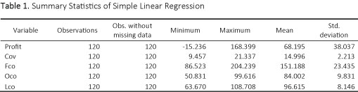
The purpose of this report is to explore how profits for 120 restaurants in a particular restaurant chain are affected by certain characteristics of the restaurants. These characteristics include number of customers served, food costs, overhead costs, labour costs, and the geographical locations where the restaurants are located. Specifically, the report will be looking at three geographical locations - Thompson Okanagan, Kootenay Rockies, and Vancouver, Coast, & Mountains. Based on these five potential predictor variables, we provide an analysis using a multiple linear regression model for predicting annual profits based on the five predictor variables.

For the rest of the report, we will be using the following abbreviations:

 Cov = number of covers or customers served (in thousands)

 Fco = food costs (in thousands of dollars)

 Oco = overhead costs (in thousands of dollars)

 Lco = labour costs (in thousands of dollars)

 Region = geographical location (1TO = Thompson Okanagan, 2KR = Kootenay Rockies, or 3VCM = Vancouver, Coast & Mountains)

Analysis 

Simple Linear Regression

To begin the analysis, we conducted a simple linear regression with the four quantitative predictors (Cov, Fco, Oco, Lco) and one categorical predictor (Region). Table 1 displays the summary statistics for the model without interactions.

Coefficient of Determination, R2

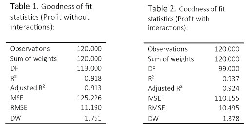
The coefficient of determination, R2, in the simple linear regression model (Table 2) is 0.918. This means that 91.8% of the total sum of squares (variation in annual profits) can be explained by using the estimated regression equation to predict the annual profits based on the five potential predictor variables.

The model was then expanded to include the interactions between the quantitative predictors and the categorical predictor. The model without interactions (Table 2) presented a lower R2 value, 0.918, than the model without interactions 0.937 (Table 3). Therefore, the second model with interactions will be used since it demonstrates a stronger linear relationship between the quantitative predictor and categorical predictor.

Residual Analysis of Model

Next a residual analysis of the model with interaction was conducted to assess the validity of the regression error assumptions. Below are the scatterplots retrieved from XLSTAT: 

Figure 1. Residual scatterplot

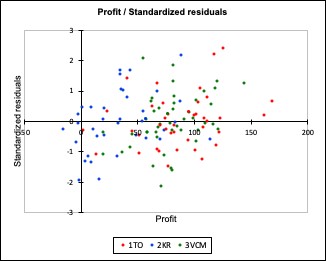
Figure 2. Normal probability plot

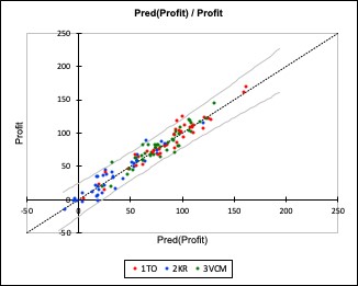
Figure 1 shows the residual scatterplot of the standardized residuals (vertical axis) versus the predicted response values, ŷ (horizontal axis). It can be characterized as a random cloud of points in a rough horizontal band. Therefore, we can conclude that the zero mean and constant variance assumptions about the errors are probably valid. 

Figure 2 is a normal probability plot of the ordered standardized residuals (vertical axis) versus normal scores (horizontal axis) with a 45o line added to the plot. It demonstrates that the data points lie reasonably close to the 45° line. Therefore, we can conclude that the error normality assumption is likely valid. Thus, we should feel comfortable drawing conclusions based on the simple linear regression analysis.

Hypothesis Testing 

In order to determine if each predictor variable is significant at a α=0.05 significance level, we must first evaluate overall significance using an F test.   

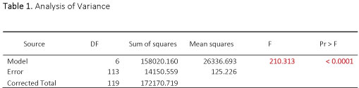
Table 4, obtained from XLSTAT, calculated the F statistic as 210.313 with a corresponding p-value 

< 0.0001. As this p-value is less than our significance level of α=0.05, we must reject the null hypothesis which suggests that there is no significant linear relationship between profit and at least one of the other predictor variables. We can then conclude that a significant linear relationship does exist between profit and one or more of the variables. Therefore, the model is better than no model. 

In order to determine which predictor variables are significant, we must conduct individual T tests to determine whether or not each predictor variable is significant based on a significance level α=0.05. 

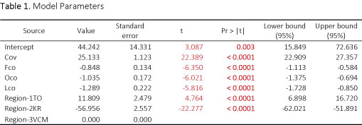
According to the model parameters in Table 5 calculated by XLSTAT, we can see that each predictor variable has t-test statistic that corresponds to a p-value < 0.0001. To calculate the Region variable the t-value test statistics are summed for Region-1TO and Region-2KR. This result allows an evaluation of the Region variable for all three regions, the resulting t-value is -17.513 with 113 degrees of freedom, resulting in a P value of < 0.0001. 

As the p-values of the remaining predictor variables are all less than the level of significance at α=0.05, we reject the null hypothesis that no significant linear relationship exists. We can conclude there is a significant linear association between each of the other predictor variables and profit, so long as all the values in the model are present and are held constant.